")
If your research project is going to involve building an SDM, then one of your first tasks will be to collate a range of different data sets so you’re all ready to do some modelling when you sit down with your supervisor (or an online tutorial, or a text book.)
That can be daunting if you haven’t had to deal spatial data before, so this is intended to be a light introduction to get you familiar with some of the more common spatial processes you might use to get everything into shape, using the two bits of software I most commonly use: ArcGIS and R. This tute was also written from the perspective of a PC user, so if you’re a Mac person that may cause some hiccups.
Please note that this is NOT intended to provide an introduction to R: if the sight of R sends you running terrified, then probably best to start somewhere else. It’s also nowhere near comprehensive, I know that, but hey, it’s a start. This doc is also pretty good if you’re planning on doing spatial stuff in R: https://cran.r-project.org/doc/contrib/intro-spatial-rl.pdf

The example we’re going to be working with is a subset of some real data from Victoria’s Central Highlands region, focussing on the Yellow-bellied glider (Petaurus australis), or the YBG as we refer to it here.
This data was collected by a team of researchers from the Victorian Department of Land, Water, Environment and Planning’s (DELWPs) Arthur Rylah Institute for Environmental Research, and was downloaded from the Victorian Biodiversity Atlas (https://vba.dse.vic.gov.au) in December 2017. The researchers used a combination of call playback and thermal imaging surveys to detect arboreal marsupials.
A bit more detail about the surveys can be found in this report:
Lumsden LF, Nelson JL, Todd CR, Scroggie MP, McNabb EG, Raadic TA, Smith SJ, Acevedo S, Cheers G, Jemison ML, Nicol MD (2013) ‘A new strategic approach to biodiversity management – research component.’ Arthur Rylah Institute for Environmental Research, Heidelberg. http://www.delwp.vic.gov.au/__data/assets/pdf_file/0007/240928/Strategic-approach-to-biodiversity-management_research-2013.pdf
This tutorial is also available as a PDF file here: Preparing spatial data for SDMs using ArcMap and R – YBG (the images in it are slightly better quality)
Table of contents
1. Download and prepare the data, and a couple of things to be aware of
-
Coordinate systems
-
Resampling data
2. Convert the CSV to points
-
ArcMap
- Displaying and symbology
-
R
4. Loading, projecting and clipping rasters, creating and buffering polygons
-
ArcMap
-
R
5. Merge polygons (line features), create a raster of distance
-
ArcMap
- Setting the Processing Environment
-
R
1. Download and prepare the data, and a couple of things to be aware of
- Create a folder on your desktop called “GIS_YBG” where all the stuff for this tute will be saved. We’re going to use five data sets: points (presence/absence of YBGs), a raster (altitude), a shapefile (old growth forest), and line features (roads). Information on the difference between these data types can be found here. The first thing you’ll need to do is download the data.
Roads (432Mb): https://www.data.vic.gov.au/data/dataset/vicmap-transport-arterial-roads
- Click ‘Order resource’, check the box, enter your email, Area type: Catchment Management Authority, select (use the right-pointing arrow) ‘Goulburn Broken’, ‘Port Phillip’ and ‘West Gippsland’, select buffer distance of 1km, Format: ESRI shape file, Projection: Geographicals on GDA94, Hit “Apply to all”, then “Submit”.
- Note: You can of course download all of Vic, I’m just trying to spare you the download wait time.
Old growth forest (4.1Mb): https://www.data.vic.gov.au/data/dataset/modelled-old-growth-boundaires
- Same process as above: just select the ‘Goulburn Broken’, ‘Port Phillip’ and ‘West Gippsland’ CMAs and a buffer distance of 1km.
Altitude (4.1Mb): This used to be available from the WordClim website (http://www.worldclim.org/tiles.php) but now the link is broken, so you can download it directly here.
- (Ignore this now – I’ve left it here in case they fix the link!)… Follow the link and select the tile we need (tile 410), some options will pop up below the map. We want GeoTIFF – Altitude.
The DataVic website will email you a link to download the data, one email per data set per CMA region (the email may take a little while to arrive).
- For roads and old growth: click on the link, and a zip file will download into your Downloads folder.
- Right click on the zip files, select ‘Extract all’ and then hit ‘Extract’ on the popup box. Once the extraction is done delete the old zip file.
Point records for Yellow-bellied gliders (YBGs) and other species
- Open this file AND save it as a .csv in your GIS_YBG folder (I just can’t attach .csv files here in WordPress). To do this go Save as > Browse (browse to GIS_YBG) > change ‘Save as type’ to CSV (comma delimited) > change the file name to “YBG_raw.csv”
Coordinate systems
Coordinate systems are far from my area of expertise, so I’m just going to touch on this briefly so I don’t leave you totally confused (more and better info here though).
There are two types of coordinate system used for spatial data which let a GIS know how to display and analyse them: Geographic Coordinate Systems (GCS), and Projected Coordinate Systems (PCS). The first is based on a 3D globe, while the latter forces our globe to be flat so we can measure things in familiar units of length and area, like hectares and metres.
This smooshing from round to flat can cause distortions, so it’s very important when transforming data based on a GCS to one based on a PCS to use a projection that is suited to the scale and location of your analyses.
So, I tend to work in a GCS like GCS GDA 1994 (which we’re using here) unless I have to measure distances or areas, in which case I convert to a PCS like VICGRID94. A projection that’s better suited to Australia-wide analyses is GDA 1994 Australian Albers.
Resampling data
There are generally three different types of inputs you might need for an SDM.
- The first is just a table with one row for each of your points, along with a column signifying whether they are an absence (a ‘0’) or a presence (a ‘1’), and columns containing the latitudes and longitudes.
- The second is a similar table, but with a corresponding column saying what the value of each your predictor variables (average amount of old growth, distance to a road and altitude in our case) is that underlies each of your points.
- If you are using a program like MaxEnt, or if you want use your model to create a map of predictions (and who doesn’t like a pretty map, right?) then you are going to need one raster for each predictor variable, and these rasters need to be EXACTLY the same coordinate system, extent, cell size, and the cells have to align perfectly.
Now, to get your rasters to all be the same then you need to do something called resampling, which I’ll show you how to do here. The thing to be aware of is that when you resample you tend to take the average from nearby cells, or cells take the values of close-by cells, and the final product can be a lot less accurate than what you started out with.
SO the take-home message here is: if you just want a table of points and the underlying values of the predictor variables, then don’t resample. If however you do want to produce a map of predictions and/or need your rasters to all be the same, then resample. This will all make a lot more sense once you get into the material below.
2. Convert the CSV to points
ArcMap
- Open ArcMap
- Save your map file by going File > Save as (navigate to GIS_YBG folder) > name the file “YBG mapping.mxd”.
- Note: This only saves your display (what data layers are showing, symbology, extent etc.) Anything you do to spatial data in Arc saves to the data file itself, SO if Arc crashes (not unheard of) all of your work is not lost – only the way you are displaying it. So crashing is very annoying, but not totally tragic. You will come to appreciate this distinction.
- Add the ArcCatalog pane by clicking this button:

- Add your GIS_YBG folder by clicking the ‘Connect to folder’ icon, and navigating to the folder.

- Navigate to your “YBG_raw.csv” file, drag and drop it into the map display area. Nothing will appear but it will show up in your ‘Table of Contents’ pane.
- Right click on the YBG_raw.csv icon, and select ‘Display XY data’.
- Make sure X Field is set to Longitude and the Y Field to Latitude. Arc Can’t automatically tell what coordinate system the CSV file is in so you need to specify this by clicking ‘Edit.’ and navigate to Geographic Coordinate Systems > Australia and New Zealand > Geocentric Datum of Australia 1994. Click OK and OK.
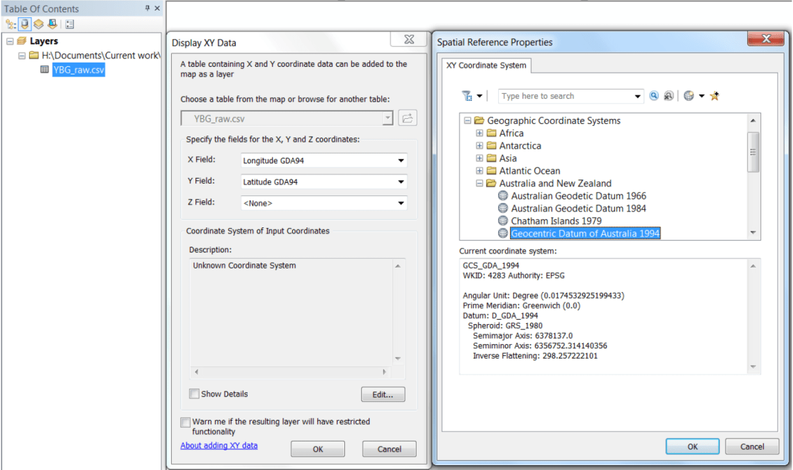
- Arc will give you a warning about Object IDs but just hit Ok.
- You can now see your data but if you look in the Table of Contents you’ll see it’s described as “Events”: this means it is being displayed but has not yet been saved as a shape file.
- Also, the coordinate system for your “Layers” data frame has now been set to GCS GDA 1994 by default because that’s what the data you’re displaying is in. This doesn’t matter so much right now, but if you add data that’s in a different coordinate system you should get warning messages and you really have to be careful if you’re doing any analysis. Something to be conscious of!
- To convert the Events to a shape (point) file: Right click on YBG_raw.csv Event, go down to Data, and then across to Export Data.. Browse to save the file as “YBGs.shp” in the GIS_YBG folder. If it asks: Yes, you want to add the exported map as a layer.
- You can now right-click on both the Events and the .csv in the Table of contents and hit ‘Remove’.
- Right-click on your YBG layer in the Table of Contents, and select Open Attribute Table: you’ll see all of the data from your original CSV displayed.
- Go the GIS_YBG folder on your desktop and have a look at how the shapefile has been saved: you’ll see a shapefile is not actually one file, but is made up of six different files (plus a lock file if you have it open in Arc at the time). If any of these get moved or corrupted the shapefile might not work properly, so it’s always best to move things around in ArcCatalog if you can.
Display and symbology
- To change the symbol of all of your points, you can just click on the icon in the Table of Contents to change the symbol, size and colour (the Symbol Selector box should pop up).
- You might like to display your points differently according to different categories in the attribute table. Let’s say we want to display the Playback and Camera records differently. To do this, right-click on the YBG layer and select Properties (last on the list).
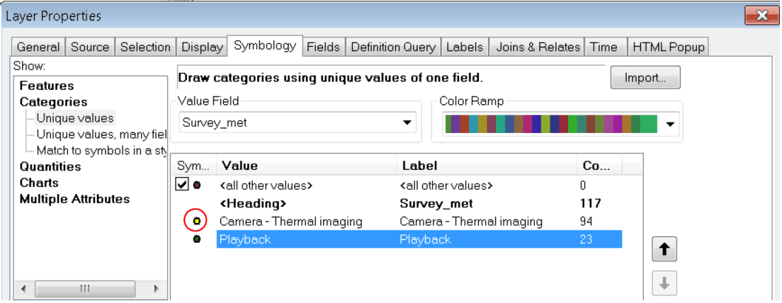
- Click on the ‘Symbology’ tab, then ‘Categories’ in the far-left pane. Under ‘Value Field’ (which is all the columns in your attribute table) select ‘Survey_met’ from the dropdown box, and then click ‘Add All Values’. Let’s make our Camera records yellow and the Playback green by double-clicking on the little symbol next to each, then changing the colour in the Symbol Selector box:
- Go back to your map. It looks like Playback has been done in fewer places: is that really the case, or are the camera records just displaying over the top? Let’s check.
- Open the YBG Attribute Table, and select “Select by attributes”:

- Double-click on ‘Survey-met’, then ‘=’, then click ‘Get Unique Values’. Double-click on ‘Playback’ when it appears. Click ‘Apply’. You’ll see all the Playback points selected.
- Close the attribute table and you’ll see the highlighted blue points are across the whole area: they’re just hiding under the yellow camera points.
- If we wanted to create a new shapefile with just these Playback points (we don’t, but just so you know) we could right-click on the YBGs layer, and go Data > Export Data, make sure “Export: Selected features” is chosen and choose where to save the new shapefile.
- Because we don’t want to do this, we are instead going to clear selected features by clicking here:

R
Note a key difference between R and Arc is that for every operation you run in Arc it will create a new file. This means that it ultimately uses up a lot more space. In R, the object won’t be saved until you do so explicitly.
Open up RStudio. Before you start, select Tools > Global Options > Code (on the left) and then make sure “Soft wrap R source files” is ticked. Copy and paste the code below into the code editing window and save the file as “GIS YBG tute” in the GIS_YBG folder.
## We'll need the raster package, so install it if you haven't already! Then load the libraries you'll need.
install.packages("raster", "rgdal", "rgeos")

library(raster)
library(rgdal)
library(rgeos)

## Set your working directory to the GIS_YBG folder
setwd("C:/Users/plentini/Desktop/GIS_YBG")

###################################################################
##################### CSV TO POINTS ###############################
###################################################################
## Load up the CSV file, call the new object "YBG_raw", tell R the table
## has a header row and is comma-separated
YBG_raw <- read.table("YBG_raw.csv", head = T, sep = ",")

## Create the spatial points from this. Specify where the x (longitude) and y (latitude) values are stored - in this case in columns 4 and 3 of the YBG_raw data frame. You'll also need to tell R what the coordinate system is (that's what the proj4string bit refers to). The table is in GCS GDA 1994, which is "+proj=longlat +ellps=GRS80 +no_defs". You can look up coordinate system codes here: http://cicero.azavea.com/docs/epsg_codes.html
YBGs <- SpatialPointsDataFrame(coords = YBG_raw[,c(4,3)], data = YBG_raw, proj4string = CRS("+proj=longlat +ellps=GRS80 +no_defs"))
## You can plot your points to have a look at them
plot(YBGs)

## Look at the attribute table
YBGs@data

## Plot just the points where the survey method is "Playback"
plot(YBGs[YBGs$Survey.method == "Playback",])

## Plot "Playback" and "Camera" in different colours. The code here says
## that if the survey method column says the point came from playback plot
## it in blue, otherwise plot it in red
plot(YBGs, col = ifelse(YBGs$Survey.method == "Playback", "forestgreen", "yellow"))

## We could create a new object with just the Playback points by giving
## the object a unique name
YBGs_playback <- YBGs[YBGs$Survey.method == "Playback",]
## Save the YBGs object as a new shape file
writeOGR(YBGs, ".", "YBGs_R", driver="ESRI Shapefile")
3. Sort the target (1) and non-target (0) species, and removing false absences
ArcMap
Our YBG data set is made up of records of both Yellow-bellied gliders and other non-target species recorded during the surveys. An approach sometimes used when building SDMs that require both presence and absence records is called ‘Target group sampling’: we know someone was in that place using a technique that should have detected an YBG but didn’t, so we can assume the presence and detection of another non-YBG species such as a Feathertail glider (Acrobates pygmaeus) equates to an absence (obviously this is a big assumption that you should think really carefully about before using in a real analysis).
- To start we’re going to project our YBGs layer, so we can more reliably measure distance in metres (instead of Decimal Degrees).
- Make sure your toolbox window is showing by clicking this icon:

- In the Toolbox select Data Management Tools > Projections and Transformations > Feature > Project.
- Select YBGs as your Input Dataset. Click on the folder next to the Output Dataset or Feature Class, navigate to the GIS_YBG folder (you can do this just by clicking on the house icon) and give the file the name “YBGs_proj”. For your Output coordinate system browse to Projected Coordinate Systems > National Grids > Australia > GDA 1994 VICGRID94 (which is second-bottom on the list). Select OK, OK.
- We’re now going to split our projected points into two data sets: those representing YBGs, or presences, and the non-YBG points, or absences.
- Right-click on the YBGs_proj layer and open the Attribute Table.
- Click on Select by Attributes.

- Double-click on Scientific, then =, then select Get Unique Values, and double-click on ‘Petaurus australis’. Click Apply, and just the YBG rows should be selected. Close the Attribute Table – we’re going to save just the highlighted points as a new shapefile.
- Right-click on the YBGs_proj layer and select Data > Export Data. The pop-up box should default to ‘Export: Selected features’, save the file as “just_YBGs_proj.shp” in the GIS_YBG folder.
- Note: If you want to see the progress/outcome of analyses like these you can bring up the Results pane by selecting Geoprocessing > Results.
- Go back into the YBGs_proj Attribute Table and reverse the selection: you do this by clicking on this icon:

- Now go back and select YBGs_proj > Data > Export Data again, but this time save your layer as “no_YBGs_proj.shp” in the GIS_YBG folder (save all outputs to this folder!)
- Clear the selection by pressing
 in the Attribute Table (or in the main console.)
 - Now, we want to make sure none of our absences (no_YBGs_proj) are within 500m of a presence (just_YBGs_proj) as these would be sitting within a home range of a Yellow-bellied glider and represent false absences. So we need to calculate how far each absence is from a presence.
- In the Toolbox select Analysis Tools > Proximity > Near. Select no_YBGs_proj as your Input features, just_YBGs_proj as your Near Features, and make sure your Search Radius is set to Metres. Click OK.

- Open the no_YBGs_proj Attribute Table, and you’ll see there are two new columns: NEAR_FID and NEAR_DIST. We want to keep all rows where NEAR_DIST is less than 500.
- In Customise > Toolbars, make sure Editor is ticked.
- Select Editor > Start Editing, and select the no_YBGs_proj layer (ignore the warning).
- In the no_YBGs_proj attribute table open Select by Attributes, double-click on “NEAR_DIST”, then <=, then type 500 into the end of the formula. Click Apply. Delete the selected rows
 , then go Editor > Stop Editing, and click ‘Yes’ when prompted to save your edits.
 - Go back into the no_YBGs_proj Attribute Table, right-click on NEAR_DIST and select ‘Delete Field’. Do the same with NEAR_FID.
- Now we need to merge no_YBGs_proj and just_YBGs proj back together, and transform them back to GCS GDA 1994. Before the next step make sure Arc will let you overwrite existing files: in the menu bar go Geoprocessing > Geoprocessing Options., and make sure the top “overwrite the outputs” box is ticked. Click OK.
- In the Toolbox select Data Management Tools > General > Merge. Select no_YBGs_proj and just_YBGs proj as your input data sets, and for the Output Dataset, save it as “YBGs_proj.shp” in the GIS_YBG folder. It will come up with an overwrite warning (because a file with that name already exists), but just click OK.
- Now transform that layer back. In the Toolbox select Data Management Tools > Projections and Transformations > Feature > Project. Select YBGs_proj as your input data set, and save your output data set as YBGs (again, you’ll need to accept the overwrite warning).
- Browse to the coordinate system you want. You can either go Geographic Coordinate Systems > Australia and New Zealand > Geocentric Datum of Australia 1994 OR simply select Layers > GCS_GDA_1994. Click OK, the OK again.
- Phew – almost there! As a final step we’re going to add a field to signify whether each row corresponds to a presence point (1) or an absence point (0).
- Right-click on the YBGs layer and open the attribute table.
- Under ‘Table options’ select ‘Add Field.’

- Call the new field ‘PA’ and for Type make it a Short Integer. Click OK.
- We want to make just the rows with ‘Petaurus australis’ equal to one, so need to select the Yellow-bellied glider points again.
- Click on Select by Attributes, and in the pop-up double-click on Scientific, then =, then select Get Unique Values, and double-click on ‘Petaurus australis’. Click Apply.
- Right-click on your new PA column (to the far right of the Table), and select Field Calculator. A warning will pop up but just click Yes. In the box at the bottom you will see that is says ‘PA =’. Type a 1 in the box, then click OK. Hey presto, your Yellow-bellied glider rows now contain a 1.
- Clear the selection by pressing
 in the Attribute Table (or in the main console).
 - See if you can figure out how to display the Yellow-bellied glider presences as purple, and the absences as blue with your new-found symbology skills.
R
Copy this code to the bottom of your existing GIS_YBG tute script file:
###################################################################
##################### SORT YOUR SPECIES ###########################
################### REMOVE FALSE ABSENCES #########################
###################################################################
# Now, before we can do any measurements we need to project our points so they're in metres, not decimal degrees. We're going to use the VICGRID94 projection for this, which is:

vicgrid <- "+proj=lcc +lat_1=-36 +lat_2=-38 +lat_0=-37 +lon_0=145 +x_0=2500000 +y_0=2500000 +ellps=GRS80 +towgs84=0,0,0,0,0,0,0 +units=m +no_defs"

# Project your points
YBGs_proj <- spTransform(YBGs, vicgrid)

# Look at the structure of the data
str(YBGs_proj@data)

# View the data
View(YBGs_proj@data)

# This will give you a list of all the unique Scientific Names in the data set
unique(YBGs_proj$Scientific.Name)

# Now let's split our Yellow-bellied glider from our non-Yellow-bellied glider points. The first line takes a subset of only those points where the species name in the attribute table is "Petaurus australis", and the second line takes only those points where it doesn't = "Petaurus australis" (that's what the ! is for)
just_YBGs <- YBGs_proj[YBGs_proj$Scientific.Name == "Petaurus australis",]
not_YBGs <- YBGs_proj[YBGs_proj$Scientific.Name != "Petaurus australis",]

# Plot that
plot(just_YBGs)
plot(not_YBGs, col = "red", add = T)

# Measure the distance of the not-YBGs from the YBGs using the 'gDistance' function
possum_dist <- gDistance(just_YBGs, not_YBGs, byid=TRUE)

# This has created a matrix of the distance of each of your 120 not-YBG points (rows) to your 16 YBG points (columns). We'll take the minimum of each row and add it to our not_YBGs data frame to see if they are less than our 500m threshold
not_YBGs@data$mindist = apply(possum_dist,1,min)

# Look at the data
View(not_YBGs@data)

# Remove rows where mindist is less than 500
not_YBGs = 500,]

# Check it
View(not_YBGs@data)

# Delete the mindist column
not_YBGs$mindist <- NULL

# Add a PA column which = 0 in not_YBGs
not_YBGs$PA <- 0

# Add a PA column which = 1 in just_YBGs
just_YBGs$PA <- 1

# Merge the two data sets back together
YBGs_proj &<- rbind(just_YBGs, not_YBGs)

# Transform them back to GCS GDA 1994
YBGs <- spTransform(YBGs_proj, YBGs@proj4string)
# Save this new 'clean' version
writeOGR(YBGs, ".", "YBGs_R", driver="ESRI Shapefile", overwrite_layer = T)
4. Loading, projecting and clipping rasters, creating and buffering polygons
ArcMap
- In ArcCatalog, navigate to the extracted altitude layer (alt_410.tif). Drag and drop it into the display window.
- Right-click on the alt_410.tif layer and select ‘Zoom to layer’ so you can see the full extent.
- Get a sense of the data. If you right-click on the layer and select ‘Properties’ and then go to the ‘Source’ tab and scroll through the information you’ll see the raster is 3600 columns × 3600 rows, is ‘float’ (so continuous rather than categorical data, which is why there is no attribute table), and the coordinate system is “GCS_WGS_1984”, which is different to our other layers. So we’ll need to fix that!
- In the Toolbox select Data Management > Projections and Transformations > Raster > Project Raster.
- Select ‘alt_410.tif’ as your input raster, your Output raster will be “alt_p” in the GIS_YBG folder, and for your Output Coordinate System navigate to Geographic Coordinate Systems > Australia and New Zealand > Geocentric Datum of Australia 1994. Click OK. When the processing is done check the Properties of ‘alt_p’: the coordinate system should be GCS_GDA_94.
- Obviously, this is more altitude data then we need, so we’re going to clip it. Let’s create a shape to specify the area that we want to clip it to.
- In the Toolbox select Data Management > Features > Minimum Bounding Geometry.
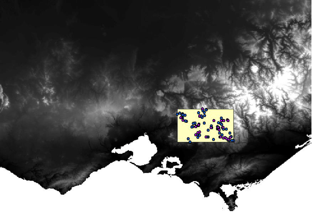
- Select Input Features: YBGs, Geometry Type: Envelope, and Group Option: All. Call the output “envelope”. Click Save and OK.
- Now you should have a map that looks something like this (I’ve zoomed in a bit here but you get the gist):
- We actually want our area to be a bit bigger than just the extent of the points in case we want to capture distance to features that are beyond this extent (such as the roads), so let’s buffer it by 5km.
- In the Toolbox, select Analysis Tools > Proximity > Buffer. Select Input features: envelope, for Output feature class say you want to save the file as “envelope_buff” in the GIS_YBG folder, set the distance value to 5km (set the dropdown box to ‘Kilometers’), and leave the rest of the field as defaults. Click ok.
- Okay – the resulting area looks a little more reasonable (right click the ‘envelope_buff’ layer and select ‘Zoom to layer’). Let’s clip the altitude raster to this.
- In the Toolbox select Data Management > Raster > Raster Processing > Clip. For Input Raster select ‘alt_p’, for the Output Extent you want envelope_buff, and you want to save the Output Raster Dataset as ‘alt’ in the GIS_YBG folder. Leave the rest as defaults.
- Hint: You can also clip shapefiles, and this Tool is found in Analysis Tools > Extract > Clip.
An alternative way to create a polygon
- You can also edit, draw and create polygons using Editing tools.
- In ArcCatalog, right-click on the GIS_YBG folder and select New > Shapefile.
- Give the file the name Study_area, make the Feature type Polygon, then choose to ‘Edit’ the coordinate system and browse to GCS_GDA_1994 like we did before.
- Click ok. The ‘Study_area’ shapefile will appear in the Table of Contents but is empty.
- Select Editor > Start Editing, and then Editor > Editing Windows > Create Features.
- Select the ‘Study area polygon’ and then ‘Rectangle’ under Construction Tools.

- Use the cursor to draw the new rectangular polygon on your map, double-click to finish drawing.
- Hint: To make you rectangle perfectly perpendicular click in the top-left corner once, then right click, then select ‘Absolute XY’, hit enter, drag cursor to bottom right corner, then double click to finish.
- Select Editor > Stop editing, and when prompted say ‘Yes’ to save your edits. That’s it! Now you can clip dtm10m_e to this if you prefer.
- You can remove ‘alt_p’ and ‘envelope’ from your Table of Contents now. You can delete them from your GIS_YBG folder too (from ArcCatalog!) if you’re feeling bold and short on space.
R
Copy this code to the bottom of your existing GIS_YBG tute script file:
###################################################################
################## RASTER MANIPULATION ############################
#################### POLYGON CREATION #############################
###################################################################

# Tell R where your downloaded "dtm10m_e" raster is: make it an object called ' altitude'
altitude <- raster("C:/Users/plentini/Downloads/alt_410_tif/alt_410.tif")

# Plot it
plot(altitude)

# Check the extent
altitude@extent

# How many columns and rows?
altitude@ncols
altitude@nrows

# Check the coordinate system
altitude@crs

# Compare that to the coordinate system of your YBG points
YBGs@proj4string # Oh dear - they look different!

# Transform the raster
alt_p <- projectRaster(altitude, crs = YBGs@proj4string)

# Check that worked
YBGs@proj4string
alt_p@crs

# Create a "bounding box" polygon around your YBG points. R has already determined what the min and max latitude and longitude are and stored it as part of the object:
YBGs@bbox

# Create a matrix with the coordinates of where you want the four corners of your new polygon, using the values in the bounding box of the YBGs object
coords <- matrix(c(YBGs@bbox[1,1], YBGs@bbox[1,2], YBGs@bbox[1,2], YBGs@bbox[1,1], YBGs@bbox[2,1], YBGs@bbox[2,1], YBGs@bbox[2,2], YBGs@bbox[2,2]), ncol = 2)

# Have a look at that, it'll make more sense
coords

# Create a non-spatial polygon with those coordinates
Poly <- Polygon(coords)

#Convert that to a SpatialPOlygon object, and tell R the coordinate system is the same as for YBGs
envelope <- SpatialPolygons(list(Polygons(list(Poly), ID = "a")), proj4string = YBGs@proj4string)

#Have a look at that
plot(envelope)

# Plot the points over the top to see if it looks about right
plot(YBGs, add = T)

# Now we can buffer that polygon. Note width = 0.05 is equal to 5km, and you want to dissolve this outside buffer area with the original polygon (otherwise you'd end up with just a ring)
envelope_buff <- buffer(envelope, width = 0.05, dissolve = T)

## Ignore the warning, we don't need the measurement to be precise.

# Have a look at that, and add the points
plot(envelope_buff)
plot(YBGs, add = T)

# If you want to have a look at it in Arc just to see if it's the same, you have to convert it to a SpatialPolygonsDataFrame first, then export it as a shapefile called "envelope_test"
envelope_buff <- SpatialPolygonsDataFrame(envelope_buff, data = data.frame(x = "data", row.names = "buffer"))
writeOGR(envelope_buff, ".", "envelope_test", driver="ESRI Shapefile")

# Now we have a buffer in the same coordinate system as the raster, so we can clip it!
altitude_clip <- crop(alt_p, envelope_buff)

# Plot it to see if it looks ok
plot(altitude_clip)

# Export it if you want to have a look at it in ArcMap
writeRaster(altitude_clip, "alt_clip_R.tiff")
5. Merge polygons (line features), create a raster of distance
ArcMap
 Add the three “TR_ROAD.shp” layers, one from each of the regions (West Gippsland, Goulburn-Broken, and Port Phillip). You’ll have to expand quite a few folders to get to these, but that’s always the case with data that comes from the Data Vic website.
- Hint: Instead of going through ArcCatalog, you can also add new layers by click on this icon:

- Now we’re going to combine the three road layers into one! Go the Toolbox and select Data Management Tools > General > Merge.
- Note: It’s often the case that you know what you want to do, but not what tool to use or where it is in the Toolbox. Even though it’s from an old version of Arc, I still find this page the most helpful in finding the name of the right Tool because of all of the handy pictures: http://webhelp.esri.com/arcgisdesktop/9.3/index.cfm?TopicName=An_overview_of_commonly_used_tools. You can also search for tools using the Search button, which looks like this:

- In the Merge window select the three TR_ROAD layers as your input data sets. For the Output Dataset, save it as “Roads.shp” in the GIS_YBG folder.
- Note: You will have to browse to each of them individually through the folder icon rather than use the drop-down menu, otherwise Arc will get narky and give you an error saying you’re using duplicate data sets:

- Click OK. This operation could take a while.
- Now we’re going to be measuring distance, which means we need to project both our roads and a template (dummy) raster. In the Toolbox select Data Management Tools > Projections and Transformations > Feature > Project.
- Select Roads as your Input Dataset, call your Output dataset “Roads_proj”, and for your Output coordinate system browse to Projected Coordinate Systems > National Grids > Australia > GDA 1994 VICGRID94 (which is second-bottom on the list). Select OK, OK.
- Do the same for the ‘alt’ raster: in the Toolbox select Data Management > Projections and Transformations > Raster > Project Raster. Select ‘alt’ as your Input Dataset, call your Output dataset “alt_proj”, and for your Output coordinate system make it GDA 1994 VICGRID94 again.
- Now create a raster that measures the distance of each cell in a raster (which is the same extent and resolution as alt_proj) to a road. In the Toolbox select Spatial Analyst Tools > Distance > Euclidean Distance.
- Note: If Spatial Analyst isn’t showing up you may need to select Customize > Extensions and check that the Spatial Analyst box is ticked.
- Set the Input raster or feature to ‘Roads_proj’, and the output distance raster as ‘roads_p_dist’ in your GIS_YBG folder.
- To make sure the output has the same extent, cell size etc. as the alt_proj layer, click on Environments. at the bottom of the tool, change the Processing extent to alt_proj, make alt_proj the Snap Raster, and change the Raster analysis: cell size to alt_proj. Click OK and it should look something like the figure below. Click OK.

- Finally, you need to transform your new distance raster this layer back to GCS_GDA_1994. In the Toolbox select Data Management > Projections and Transformations > Raster > Project Raster. Select ‘road_p_dist’ as your Input Dataset, call your Output dataset “roads_dist”, and for your Output coordinate system make it GCS_GDA_1994.
- It’s a bit hard to see the detail in the resulting layer, so to make this clearer right click on ‘road_dist’ and select Properties. Go to the Symbology tab, and click on the ‘Classify.’ button. Under Classification Method, select Quantile from the drop-down menu, then click OK.
- Done! You can now remove the three ‘TR_ROAD’ layers, alt_proj, Roads, Roads_proj, and roads_p_dist.
Setting the Processing Environment
Now, before progressing any further we’re going to set the Processing Environment. This means that for every geoprocess that we run (i.e. every tool we use) it will only work across the extent that we specify, and any output raster will have the same cell size, extent and alignment as a raster that we specify. This is basically the equivalent of resampling for every raster process we run from here on, which comes with the issues I noted above!
We’re going to use the ‘alt’ raster as our template.
- From the top menu select Geoprocessing > Environments.
- Under ‘Processing Extent’ set the Extent to ‘Same as layer alt’ from the dropdown menu, and the Snap Raster to ‘alt’ also. Under ‘Raster Analysis’ set the Cell Size to ‘Same as layer alt’. Leave everything else as is. Click OK.

R
Copy this code to the bottom of your existing GIS_YBG tute script file:
###################################################################
################## MERGE LINE FEATURES ############################
################# CREATE DISTANCE RASTER ##########################
###################################################################
# First a warning: this part of the tute will take a while! Be patient, have a cup of tea, read a paper. And don't remove stuff from your workspace as I do if you're not entirely sure if it's worked, esp. if it takes yonks to load.

# Load up your three 'TR_ROAD' layers, direct R to where you downloaded them (yours may or may not have "1000" in the directory)
GB_rd <- shapefile("C:/Users/plentini/Downloads/SDM375271/ll_gda94/shape/cma100/goulburn broken-1000/VMTRANS/TR_ROAD.shp")
PP_rd <- shapefile("C:/Users/plentini/Downloads/SDM375271/ll_gda94/shape/cma100//port phillip and westernport-1000/VMTRANS/TR_ROAD.shp")
WG_rd <- shapefile("C:/Users/plentini/Downloads/SDM375271/ll_gda94/shape/cma100//west gippsland-1000/VMTRANS/TR_ROAD.shp")

# Plot them over
"green") # pch is the 'plotting character', and 21 is a circle
plot(WG_rd, add = T, col = "dodgerblue") # Yup, doesn't look right
plot(PP_rd, add = T, col = "forestgreen")
plot(GB_rd, add = T, col = "maroon4") # Not Maroon5, never maroon5

# Merge your three road layers
Roads <- rbind(WG_rd, PP_rd, GB_rd)

# Plot it to check
plot(Roads)

# Clip the roads to your study area
roads_clip <- Roads[envelope_buff, ]

# Did that work?
plot(roads_clip)

# Remove the original three layers from your workspace
rm(GB_rd, PP_rd, WG_rd)

# While we're at it, let's get rid of all the other unnecessary stuff too!
rm(coords, YBG_raw, possum_dist, altitude, altitude_proj, envelope, envelope_buff, just_YBGs, YBGs_playback, YBGs_proj, not_YBGs, Poly, Roads)

# Now, before we can do any measurements we need to project both the roads and the raster so they're in metres, not decimal degrees. We're going to use the VICGRID94 projection again for this.

# Project your roads
roads_vicgrid <- spTransform(roads_clip, vicgrid)

# We also need a dummy raster to work from - we'll use the altitude_clip layer for this
dummy <- altitude_clip

#Project your dummy raster
dummy_vicgrid <- projectRaster(dummy, crs = vicgrid)

# Check it
roads_vicgrid@proj4string
dummy_vicgrid@crs #Looks good

# The function we're going to use won't work if we've got NoData in our raster, so let's check:
summary(as.data.frame(dummy_vicgrid, na.omit=T))

# Looks like there are 2324 NoData values, so let's replace those with 0s
dummy_vicgrid[is.na(dummy_vicgrid)] <- 0

# Check again
summary(as.data.frame(dummy_vicgrid, na.omit=T)) # Better!

# Now we can create the distance raster. This function converts your raster to SpatialPoints (one point for the centroid of each cell), then measures the distance of each of these points to each road (so it takes a while).
road_dist <- gDistance(roads_vicgrid, as(dummy_vicgrid,"SpatialPoints"), byid=TRUE)

# Fill each cell of the dummy raster with the distance to the road that was closest (the minimum of all measurements taken)
dummy_vicgrid[] = apply(road_dist,1,min)

# Plot it to see if it looks okay
plot(dummy_vicgrid)

# Now transform it back to GCS GDA 1994, and save the .tiff
roaddist_raster <- projectRaster(dummy_vicgrid, crs = YBGs@proj4string)
writeRaster(roaddist_raster, "roaddist_raster_R.tiff")

# Remove stuff you no longer need
rm(dummy, dummy_vicgrid, road_dist, roads_vicgrid, roads_clip)
6. Delete polygons, convert them to a raster, manage NoData, create a raster of averages
ArcMap
Next we’re going to calculate the average amount of old-growth forest within a kilometre of each grid cell.
- Add the three “MOG2009.shp” layers, one from each of the regions, just so you can get a sense of the data you’re working with.
- To do the calculations, we first need to merge our three shapefiles into one, like we did with our roads. In the Toolbox select Data Management Tools > General > Merge.
- Remember we need to browse to the layers, so click on the little folder icon and select each of the MOG2009 layers one by one. Call the output data set “old_growth”, make sure you’re saving it in the GIS_YBG folder. Click OK.
- Right-click on the old-growth layer, and open up the attribute table to have a look at it. In the X_OGCODE field you’ll see that this layer actually contain both “Old growth forest” and “Not old growth forest” (who knows why). We don’t want the non-old growth, so let’s delete them!
- Close the Attribute Table, and get yourself into editing mode by clicking Editor > Start Editing.

- In the popup box that appears, double click on the old_growth layer.
- Now open up the old-growth Attribute Table again and Select by Attributes.

- Double-click on “X_OGCODE”, then ‘=’, then “Get Unique Values”, and then ‘Not Old Growth Forest’, then click Apply. You’ll see all the ‘not old growths’ have been highlighted.
- Delete them by clicking on the Delete Selected symbol:

- Now all of your features should have the same OGCODE (1).
- Close the Attribute Table (you’ll see there are now fewer polygons in the layer), and select Editor > Stop editing. When it asks if you want to save your edits say ‘Yes’.
- Now we can convert our polygons to a raster!
- In the Toolbox select Conversion Tools > To Raster > Polygon to Raster.
- Your Input Features will be old_growth, the Field you are basing your conversion on will be ‘OGCODE’ (so the raster you produce will have a ‘1’ for old growth areas and NoData elsewhere) and call your Output raster “oldgrowth”. Click ‘OK’.
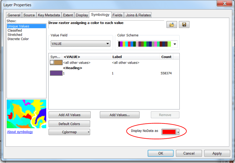
- You’ll see in the resulting raster (which might be hiding under your old_growth polygons so you might have to turn them off) that there are only colours where old_growth was equal to one: everything else is clear. This is because the other cells contain NoData values (kind of like ‘NA’ in a data set) which can stuff up calculations.
- If you right-click on the oldgrowth raster and select Properties > Symbology, you’ll see down the bottom-right corner that you can choose to “Display NoData as”. Let’s make it red, and click OK.
- Now you can see you’ve actually got a raster that is the same extent/resolution as the altitude raster (because we set the Processing Environment). Instead of NoData values, we want these to be 0’s for the sake of our calculations. Let’s fix that.
- In the Toolbox select Spatial Analyst Tools > Reclass > Reclassify.
- Select ‘oldgrowth’ as your Input raster. Arc will automatically set the Reclass field to ‘VALUE” (which is correct) and populate the Reclassification table. You want to manually change where it says ’NoData’ in the New Value field to 0, and name the Output raster “oldgrowth01”. Click OK.

- Now we have a raster made up of 0s and 1s that we can base our average calculations on.
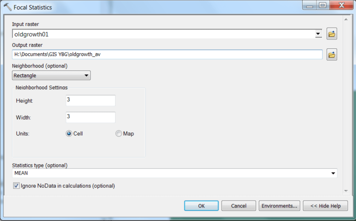
- In the Toolbox select Spatial Analyst Tools > Neighbourhood > Focal Statistics.
- Select oldgrowth01 as your input raster, and call the Output raster oldgrowth_av. We’re going to calculate our average within an ~833km radius of each cell, because the cells in our raster are ~833m × ~833m (see the layer’s Properties > Source, Cell Size is three rows down).
- Select the Neighbourhood to be calculated as a “Rectangle”, and it’ll default to 3 × 3, which looks this:

Hence, a 3 × 3 rectangle is the equivalent of taking the average of 833m around each cell. If we wanted a 1.6km radius for example, we’d need to set our rectangle to 5 × 5 (a centre column, then 2 × 833m cells to the left and right of that). That’s as clearly as I can explain that ![]()
- And now you have your average amount of Old Growth raster! Remember to remove things from your work space as you go along to remove clutter: you really only need road_dist, alt, oldgrowth_av, and YBGs at this point.
R
###################################################################
#################### POLYGONS TO RASTER ###########################
#################### RASTER OF AVERAGES ###########################
###################################################################
# Load up your old growth data from the three CMA folders
GB_og <- shapefile("C:/Users/plentini/Downloads/SDM374386/ll_gda94/shape/cma100/goulburn broken-1000/FORESTS/MOG2009.shp")
PP_og <- shapefile("C:/Users/plentini/Downloads/SDM374386/ll_gda94/shape/cma100/port phillip and westernport-1000/FORESTS/MOG2009.shp")
WG_og <- shapefile("C:/Users/plentini/Downloads/SDM374386/ll_gda94/shape/cma100/west gippsland-1000/FORESTS/MOG2009.shp")

# Merge those
old_growth <- rbind(WG_og, PP_og, GB_og)

# Plot it to check
plot(old_growth)

# Look at the underlying attribute table/data
old_growth@data

# You can see those pesky "not old growths". Let's delete them -  this bit of code tells R to only keep the rows that have exactly "Old Growth Forest" in the X_OGCODE column
old_growth <- old_growth[old_growth$X_OGCODE == "Old Growth Forest",]

# Look at the data again
old_growth@data #Better!

# Convert this shape file to a raster, using the altitude_clip raster as a template
oldgrowth_raster <- rasterize(old_growth, altitude_clip)

# Plot it to check
plot(oldgrowth_raster) # The blank bits are the NAs/NoData values

# If you look at the summary data you'll see it's retained all four attributes (and is plotting Hectares)
summary(as.data.frame(oldgrowth_raster))

# We only want a binary 'old growth or not' raster, so let's convert all the real (non-NA) values to 1s first:
oldgrowth_raster[!is.na(oldgrowth_raster)] <- 1

# And now let's make the NAs = 0
oldgrowth_raster[is.na(oldgrowth_raster)] <- 0

# Plot it to check
plot(oldgrowth_raster)

# Now calculate an average across a 3 * 3 matrix around each cell
oldgrowth_av<- focal(oldgrowth_raster, w = matrix(rep(1, 9), ncol = 3, nrow = 3), fun=mean, na.rm = T)

# Plot it
plot(oldgrowth_av)

# Good. Now write the .tiff
writeRaster(oldgrowth_av, "oldgrowth_av_R.tiff")
7. Prepare your data: extract data from points, resample and export rasters to ASCII
To recap what I said at the beginning, there are different outputs you might want from all of this:
- A table with one row per point, a column signifying whether points are absences or presences, and columns containing the latitudes and longitudes.
- A table that also has columns with the values of the predictor variables underlying each point.
- One raster for each predictor variable, each with the same coordinate system, extent, cell size etc.
ArcMap
- If you just want a table with presences, absences, lats and longs, then you already have that. Just open the YBGs Attribute Table, and under Table options (
 ) select Export…
 - Browse to save the output. Change the format to ‘Text file’, and call the file “YBGs01.csv” (note to change the extension). Click Save, OK.

- You can open this file in Excel from the GIS_YBG folder if you’d like to have a look at it.
- Let’s add the predictions from the rasters to the Table. In the Toolbox select Spatial Analyst Tools > Extraction > Extract Multi Values to Points.
- Select ‘YBGs’ as your Input point features and for ‘Input rasters’ you can select ‘road_dist’, ‘alt’, and ‘oldgrowth_av’ from the dropdown menu. Click OK.
- Once the tool is done you can open up the YBGs Attribute Table and will see the three extra columns corresponding to the three predictors. You can export this in the same fashion above if you like.
- Note: You can also extract the value of a polygon at each point by right-clicking on your point layer, then selecting Joins and Relates > Join…, then select ‘Join data from another layer based upon spatial location’ from the drop down menu in the dialog box. But this is a lot easier to do in R (see below).
- Now, because we set our Processing Environment in theory our three rasters should all have the same cell size and have the same extent, cell size etc. Let’s check. Open the road_dist Properties, and click on the Source tab. It says this raster has 129 columns, 80 rows, and the cell size is 0.0085032718. Do the same for the ‘alt’ raster: it has 129 columns, 79 rows, and the cell size is 0.0083333333. Drat – we’ll have to fix that! ‘old_growth’ on the other hand seems to be behaving itself.
- In the Toolbox select Data Management Tools > Raster > Raster Processing > Resample.
- In the popup set road_dist as your input, call your output “road_resample”, and make sure you set the Output Cell Size to ‘Same as layer alt’:

- Check the properties of the resulting ‘road_resample’ layer: ugh, now it says 129 columns and 80 rows (but the cells size is correct). So we still have one extra row. It happens: this step is usually mega frustrating. Okay, let’s try clipping it. Tools > Data Management Tools > Raster > Raster Processing > Clip. Make the input ‘road_resample’, set the output extent to ‘alt’, and call the output ‘road_res’. Click OK.
- Check the Properties of the road_res output: Yaaaay, that worked! Thank god for that. Now we can export our rasters to ASCII.
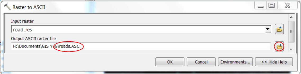
- In the Toolbox select Conversion Tools > From Raster > Raster to ASCII.
- You’ll need to run the tool three times, one for each predictor (road_res, oldgrowth_av and alt). Make sure that for where it says “Output ASCII” you browse and in the popup box change the format from .txt to .asc, and that the extension for the output is .asc:
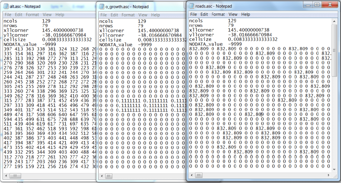
- You can open the ASCIIs in a text editor to check the rows at the top all match. If they do, then they are ready to go 🙂
R
Copy this code to the bottom of your existing GIS_YBG tute script file:
###################################################################
##################### SAMPLING POINTS #############################
#################### RESAMPLING RASTERS ###########################
###################################################################

# If we want to just export the YBGs table as a csv, it's as simple as
write.table(YBGs@data, file = "YBGs01_R.csv", sep = ",", row.names = F)

# We can then sample the predictor values from our points one at a time
OG <- extract(oldgrowth_av, YBGs)
RD <- extract(roaddist_raster, YBGs)
ALT <-- extract(altitude_clip, YBGs)

# Note: if you want to extract the value of a polygon (instead of a raster) underlying a point you can use the 'over' function, for example:
pointvalues <- over(YBGs, old_growth)

# Add those to the YBGs table
YBGs@data$OG <- OG
YBGs@data$RD <- RD
YBGs@data$ALT <- ALT

# Now you can export that
write.table(YBGs@data, file = "YBGs_preds_R.csv", sep = ",", row.names = F)

# Check the extent, resolution, dimensions, and coordinate system of your rasters
area(oldgrowth_av)
area(roaddist_raster) # Looks different
area(altitude_clip)

# We'll have to resample the roaddist_raster
roaddist_res <- resample(roaddist_raster, altitude_clip)

# Check everything again
area(oldgrowth_av)
area(roaddist_res) # Looks better!
area(altitude_clip)

# Export the rasters as ASCIIs
writeRaster(oldgrowth_av, file = "OG_R.asc")
writeRaster(roaddist_res, file = "RD_R.asc")
writeRaster(altitude_clip, file = "ALT_R.asc")

########################### FIN ###################################
I hope at the end of this you’ve noticed a few things: firstly, some processes work faster in R, and some in Arc. It can help to develop an understanding of which does what better/in a more intuitive way. I generally prefer Arc for visualisation and R for actual analysis and processing, but each to their own.
You should also notice that by going through Arc you create a whole lotta interim shapefiles and rasters that you don’t actually need but take up lots of space. R doesn’t create this problem.
Finally, if you find a small error in your data set (which you inevitably will), in R you can change the input data and will the click of a button can rerun your whole spatial analysis. If you’ve done your work in Arc, you’re going to have to go through the whole pointy-clicky-creating-things-I-don’t-need process again that leads to major time suckage and stress. Take care of future you, and try and avoid this as much as possible!

This is great Pia. Really useful resource!